
Abstract
The UKCS Central Graben plays host to some of the most prolific of the Palaeocene and Eocene North Sea turbidite systems. The interval can be broadly sub-divided into three main fan building episodes, namely Andrew/Lista, Forties/Sele and the younger Tay Fan system. This study focuses on the middle to upper Tay sands which are found in a number of channel-lobe complexes in block 21/23 UKCS. Individual channels may be as small as 2-300m across and up to 50m thick, retaining a relatively linear, low sinuosity morphometry. Lateral stacking, erosion and bypass are common features observed on both well and seismic scales and can result in amalgamated sand bodies which may reach several hundred feet in thickness.
The first part of the paper discusses the history of Oilexco's Sheryl discovery. Two wells with a total of 10 legs penetrate the Sheryl discovery. The reservoir was tested with the last leg and had a maximum rate of more than 1900 BOPD oil.
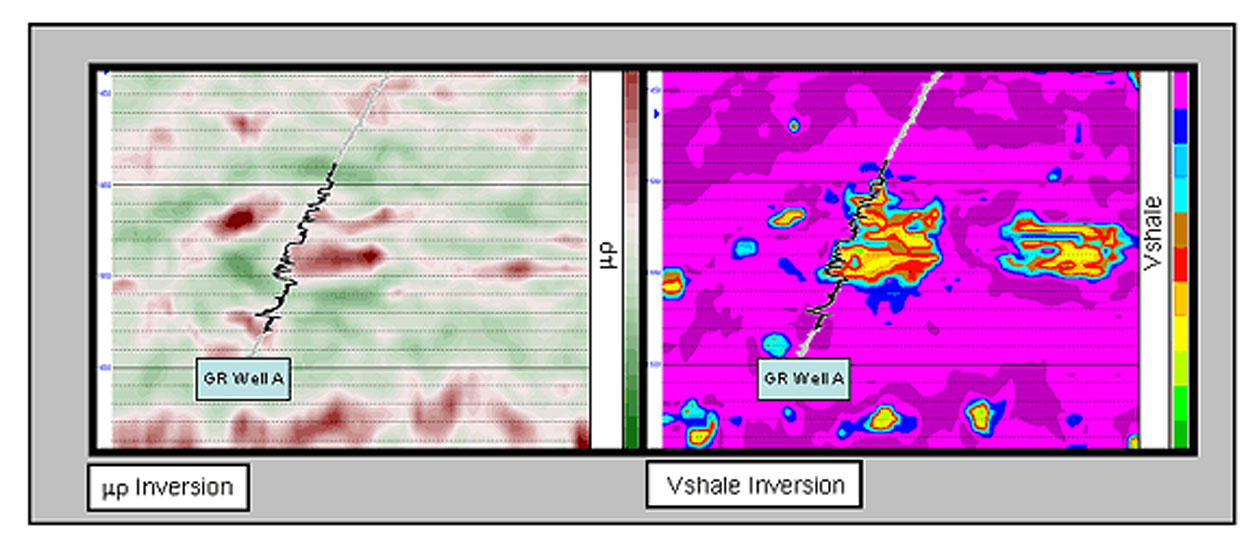
While the first wells were drilled on far stack amplitude and elastic impedance anomalies, the second set of wells were placed using an added LMR inversion. Rock physical analysis of the existing well data revealed that the sands in the Tay system are generally harder than the overlying shale. However, under the influence of hydrocarbons, the acoustic properties of the sands become similar to overlaying shale or even softer. Independent of this trend, the shear modulus for sand was generally higher than for the bounding shales, and therefore, MR mapping warranted an improved sand identification. At the end of the drilling period a set of Vshale logs derived from the well data served as a target variable to train neural network to refine the reservoir mapping (fig.1).
Even though a good workflow for sand mapping was established, the hydrocarbon identification remained a challenge. In particular the difference in the OWC on the East and West flanks of the field was puzzling. To find a the solution for this problem, higher resolution seismic data was necessary. The ThinMAN inversion process delivered a tool to refine the interpretation, and allowed the identification of individual connected or disconnected sand layers. The high resolution ThinMAN reflectivities enabled the interpreter to map the OWC, which is expressed by a flat spot on the high resolution ThinMAN reflectivities. Furthermore, it was found that the ThinMAN data set could be tied with high confidence to key biostratigrafic intervals. At the end of the workflow a reliable map of the sand was mapped and significant upside potential within the development area could be established.
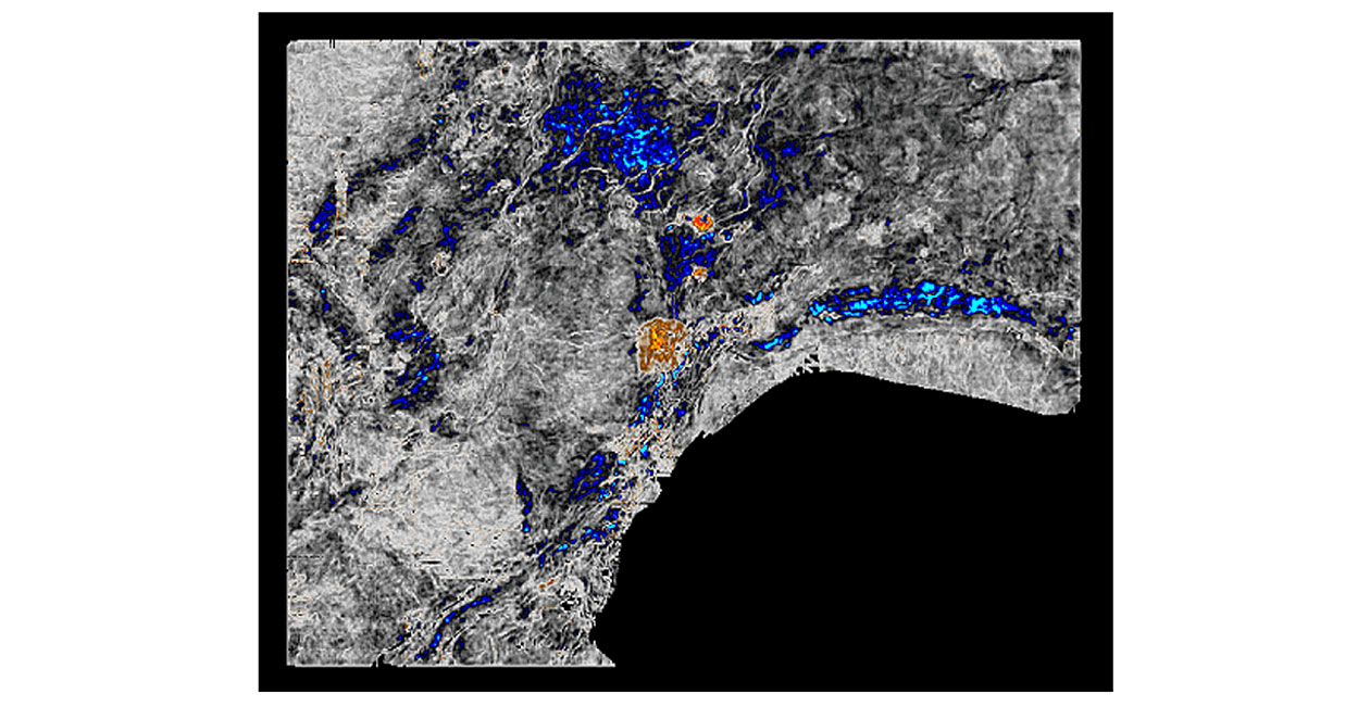
The second part of the presentation discusses how the lessons learnt during the Sheryl discovery are applied to a new exploration area some 8km to the NE. In this area a remarkable channel amplitude anomaly captured the attention of the interpreters (fig.2). Before the Sheryl wells were drilled, this area was devaluated because extensive modeling with a number of 2D stratigraphic AVO near and far stack models for brine, oil and gas bearing reservoir, indicated a small chance of success of finding hydrocarbon bearing reservoir in the main anomaly. However, being in the possession of a detailed template database after the Sheryl discovery and other wells in the vicinity, additional LMR analysis and mapping indicates the possibility of HC filled sand. One of the templates is illustrated in figure 3. Figure 4 shows a seismic section through one of the side channels and the corresponding LMR interpretation. In the near future the drill bit will be the "hard test" for the interpretation.
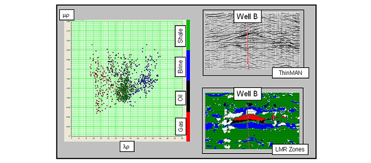
a) LMR crossplot; samples are extracted from the 3D seismic around the template Well B and color-coded for the fluids.
b) ThinMAN inversion, GOC and OWC are apparent as flat lines.
c) LMR crossplot section, color-coded according to figure 3a.

Note: The blue (brine) points above the zone of interest are a result of overlapping "brine" and "shale" zones.
Biography
Biography unavailable.